PythonPythonME

Machine learning

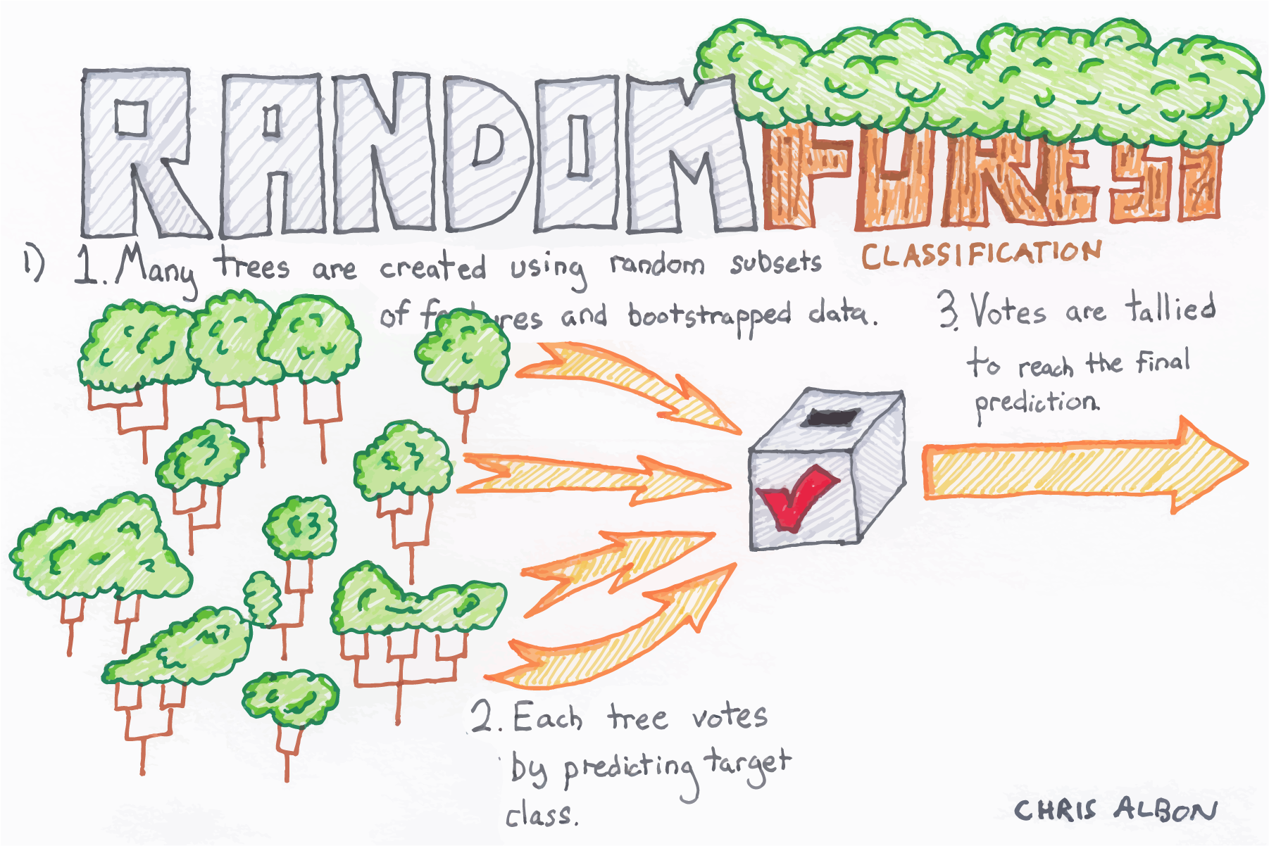
Random Forrest:

Using several decision trees and combining their predictions, the ensemble learning algorithm Random Forest creates a more accurate and reliable model.

It operates by building a collection of decision trees during training and then displaying the mean prediction (regression) or the mode of the classes (classification) for each tree.

Two kinds of randomness are used by Random Forest:

Randomness in the data points chosen for each tree's training (Bootstrap aggregating, or bagging)

Randomness in the selection of the features that are used to divide each node in a tree (for each tree, a subset of all the features available is chosen).

Random Forest's primary benefits are:

Due to the combination of many trees and eliminating overfitting, the accuracy and resilience are high.
being able to manage a variety of input features
can perform problems involving both classification and regression

The following are the primary drawbacks of Random Forest:

Compared to simpler models like linear regression, the model's output requires more interpretation.
When dealing with large datasets or a lot of trees, it might be slow and costly in terms of computing.
On unbalanced datasets, it might not perform well.

A demonsration is shown below :

Codeblock E.1. Decision tree demonstration.

Overview Random Forest - gaussian37

Figure E.1. A Random forrest in ML.

You can download this Ipynb file from here :

Download. Download the Random forrest.ipynb files used here.

The second part of that looks like this :

from sklearn.datasets import load_iris
from sklearn.ensemble import RandomForestClassifier
from sklearn.model_selection import train_test_split
from sklearn.metrics import accuracy_score, confusion_matrix
import matplotlib.pyplot as plt
import seaborn as sns

# Load the Iris dataset
iris = load_iris()
X = iris.data
y = iris.target

# Split the dataset into training and testing sets
X_train, X_test, y_train, y_test = train_test_split(X, y, test_size=0.3, random_state=42)

# Create an instance of the RandomForestClassifier class
clf = RandomForestClassifier(n_estimators=100, random_state=42)

# Fit the classifier to the training data
clf.fit(X_train, y_train)

# Make predictions on the testing data
y_pred = clf.predict(X_test)

# Evaluate the accuracy of the classifier
acc = accuracy_score(y_test, y_pred)
print("Accuracy:", acc)

# Plot the confusion matrix
cm = confusion_matrix(y_test, y_pred)
sns.heatmap(cm, annot=True, cmap='Blues')
plt.xlabel('Predicted')
plt.ylabel('True')
plt.title('Confusion Matrix')
plt.show()

# Plot the feature importances
feature_importances = clf.feature_importances_
sns.barplot(x=feature_importances, y=iris.feature_names)
plt.xlabel('Feature Importance Score')
plt.ylabel('Features')
plt.title('Feature Importances')
plt.show()

Figure E.1. Confusion matrix for Iris data.

---- Summary ----

An ensemble learning approach called Random Forest mixes various decision trees to produce a highly accurate and generalizable model. To describe Random Forest, consider the following main points:

A group of decision trees called Random Forest uses an average of each tree's forecasts to produce predictions.
Each decision tree is trained on a different subset of the training data created by Random Forest using a method called bagging.
Additionally, each split in each decision tree is assigned a subset of features by Random Forest using a method called feature bagging.
An efficient technique for classification and regression applications, Random Forest is frequently used to resolve challenging issues.
With Random Forest, overfitting is minimized, missing values and outliers are handled, and feature relevance rankings are provided.
Additionally, Random Forest has significant drawbacks, such as being computationally expensive and challenging to understand, particularly for large datasets with numerous features.