PythonPythonME

Machine learning

Decision Trees:

In machine learning, decision trees are a particular supervised learning technique used for both classification and regression tasks.

They operate by dividing the input space into a number of rectangles, each of which represents a section of the input space and has a label.

By posing a series of inquiries with the goal of lowering the level of ambiguity surrounding the target variable, input space is segmented.

A root node, internal nodes, and leaf nodes make up a decision tree.

Each internal node represents a test on an attribute, whereas the root node represents the complete dataset.

The leaf nodes represent the classes or the regression values, while the edges represent the test result.

Every connection between a leaf node and the root node represents a decision rule.

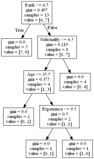
Python Machine Learning Decision Tree

Figure E.1. A Decision tree in ML.

The top-down decision tree learning technique divides the data into subsets until all samples in a subset are members of the same class or have the same value.

To build the decision tree, the algorithm selects the characteristic that offers the most information gain or the best split at each node.

Decision trees can handle both numerical and categorical data and are simple to comprehend and analyze.

They can also deal with data outliers and missing numbers.

Overfitting in decision trees can be avoided by trimming the tree or employing ensemble techniques like Random Forests.

A demonsration is shown below :

Codeblock E.1. Decision tree demonstration.

The following Python code illustrates how to utilize the Decision Tree Classifier function from the scikit-learn library:

import load_iris from sklearn.datasets to load the Iris dataset from the datasets that come with scikit-learn.

import from sklearn.tree The Decision Tree Classifier model is imported by DecisionTreeClassifier from the tree module of Scikit-Learn.

In order to divide the dataset into training and testing sets, the train_test_split function from the model_selection module is imported from sklearn.model_selection.

from sklearn.metrics import accuracy_score: Imports the accuracy_score function to assess the classifier's accuracy.

plot_tree is imported from the tree module in sklearn.tree in order to plot the decision tree.

The Iris dataset is loaded into the iris variable by using load_iris().

Separate the features and target from the dataset by writing X = iris.data and y = iris.target.

The formula train_test_split(X, y, test_size=0.3, random_state=42) divides the dataset into training and testing sets, with 30% of the data being utilized for testing.

clf = DecisionTreeClassifier(random_state=42) creates a DecisionTreeClassifier object with the value 42 for random_state.

Fits the classifier to the training set of data using clf.fit(X_train, y_train).

The target variable for the testing dataset is predicted by the formula y_pred = clf.predict(X_test).

Calculates the accuracy of the classifier using the formula acc = accuracy_score(y_test, y_pred).

Plots the decision tree using the plot_tree function with the filled parameter set to True, which colors the nodes in accordance with the majority class. The syntax is plot_tree(clf, filled=True).

The resultant graph looks like this :

Figure E.1. Decision tree generated.

You can download this Ipynb file from here :

Download. Download the Decision trees.ipynb files used here.

The second part of that looks like this :

from sklearn.datasets import load_iris
from sklearn.tree import DecisionTreeClassifier, plot_tree
from sklearn.model_selection import train_test_split
from sklearn.metrics import accuracy_score, confusion_matrix
import matplotlib.pyplot as plt

# Load the iris dataset
iris = load_iris()
X = iris.data
y = iris.target
target_names = iris.target_names

# Split the dataset into training and testing sets
X_train, X_test, y_train, y_test = train_test_split(X, y, test_size=0.3, random_state=42)

# Create an instance of DecisionTreeClassifier
clf = DecisionTreeClassifier(max_depth=2)

# Fit the classifier to the training data
clf.fit(X_train, y_train)

# Make predictions on the testing data
y_pred = clf.predict(X_test)

# Evaluate the accuracy of the classifier
acc = accuracy_score(y_test, y_pred)
print("Accuracy:", acc)

# Plot the decision tree
plt.figure(figsize=(10, 8))
plot_tree(clf, filled=True, feature_names=iris.feature_names, class_names=target_names)
plt.show()

# Compute and plot the confusion matrix
cm = confusion_matrix(y_test, y_pred)
fig, ax = plt.subplots()
im = ax.imshow(cm, cmap=plt.cm.Blues)
ax.set_xticks([0, 1, 2])
ax.set_yticks([0, 1, 2])
ax.set_xticklabels(target_names)
ax.set_yticklabels(target_names)
ax.set_xlabel("Predicted")
ax.set_ylabel("True")
ax.set_title("Confusion Matrix")
plt.colorbar(im)
plt.show()

Figure E.1. Decision tree for Iris data.

---- Summary ----

A well-liked machine learning approach for classification and regression tasks is decision trees.

They function by repeatedly dividing the data into subsets according to the value of a single feature, resulting in a model that resembles a tree and predicts the target variable.

The following are some essentials to keep in mind when using decision trees:

They are helpful for outlining the thinking behind forecasts since they are simple to comprehend and interpret.
Both numerical and categorical data can be handled by them.
They might be more prone to overfitting if the dataset is small or the tree is overly complicated.
Overfitting can be avoided by pruning, limiting the depth of the tree, or requiring a minimum number of samples per leaf.
Decision trees' use of surrogate splits allows them to accommodate missing data.
Entropy and the Gini index are two examples of impurity measurements that can be used to gauge the quality of a split.
A diagram of a tree can be used to represent decision trees.
Decision trees perform better when using ensemble approaches like random forests and gradient boosting, which reduce overfitting and combine several weak classifiers.